by Roberto Cimadevilla and Javier Garcia-Villalobos, ZIV, Spain
The use of line differential protection has been spreading more and more due to the increased availability of communication channels with adequate bandwidth. Line differential protection provides important advantages over distance protection such as better resistive coverage; good dependability for cross-country faults, selectivity protecting short lines, unaffected by: power swings, voltage inversions in series compensated lines, mutual coupling in parallel lines, load encroachment, etc. However, line differential relays may be affected by several adverse conditions such as severe CT saturation, SDH switching, very high resistive faults, high capacitive current, communication errors.
Line Differential Relay Based on Instantaneous Values
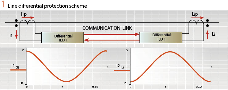
Review of the operating principle of a line differential protection: A line differential protection system is based on several IEDs, each of them located at one end of the protected line. To simplify the explanation, the two-ended line of Figure 1 is considered. Each of the IEDs measures the local current and receives, via the communication channel, the currents measured by the remote IED. The local IED calculates the differential and restraint currents using the following formulas:
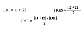
The local IED samples the current at several time instants, as it is shown in Figure 2. The current can be measured as instantaneous values or phasors. The remote IED must sample the current at the same time instants. Any synchronization error in the time instants will generate a false differential current.
Advantages of using instantaneous values instead of phasors: Line differential relays based on instantaneous values present several advantages over the ones using phasors. Some are detailed below.
Calculation of the harmonics in the differential current: This calculation allows the protection of groups line plus transformer or even transformers alone. The first application is required when, because of economic reasons, there is no breaker between the line and the power transformer and both elements must be protected by the same differential relay. The second application is needed when the distance between the CTs in the first and the second windings is very long. This requires very long wires, creating an excessive burden in one of the CTs, limiting the use of a transformer differential protection.
It is important to note that harmonic blocking or restraint units require the use of the harmonics present in the differential current. If the units are based on the harmonics present in the first winding currents, the operation may not be correct for inrush or overexcitation conditions that occur with the transformer loaded, as the harmonic content in the first winding currents may be much lower than the one included in the differential current. Inrush with the transformer loaded can occur when clearing an external fault or during a sympathetic inrush. If just the phasors at the fundamental frequency are interchanged between both line differential IEDs the harmonic information of the remote end currents is lost.
Calculation of the restraint current based on TRUE RMS values:
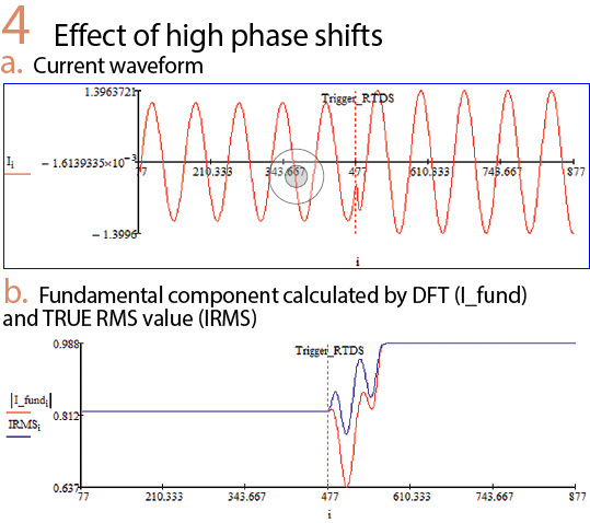
Restraint current based on TRUE RMS value provides better security than using just the fundamental component. TRUE RMS value is slightly higher than the fundamental component during symmetrical CT saturation and it is much higher than the fundamental component during asymmetrical CT saturation, because of the DC offset. On the other hand, TRUE RMS value is not affected by high phase shifts between prefault and fault currents, which causes the DFT to transiently calculate a current lower than the prefault one. Figure 4a shows a current that has experienced, due to the fault, a high phase shift. Figure 4b shows the fundamental component of the current calculated by a DFT and the TRUE RMS value. It can be seen that the DFT calculation transiently decreases, giving very low current values. The calculated TRUE RMS gives much higher values during the transient state.
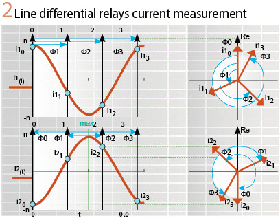
Use of an external fault detector based on the instantaneous ratio idifferential / irestraint: ZIV transformer and busbar differential relays include, since many years ago, an external fault detector which operates when the ratio between the instantaneous differential and restraint currents is below a threshold (k). When the fault is external, during the time the CT is not saturated, the ratio is very small. Figure 3 (a/b/c) shows, for an external fault, the phase A currents in line ends 1 and 2 and the instantaneous differential and restraint currents. This external fault makes the CT in line end 1 saturate. As it can be observed, since the activation of a fault detector (signal FDET, based on current change), there is a consecutive number of samples with a very low idif/ires ratio. If this happens, the external fault condition is activated.
This unit can also be included in line differential relays. As it calculates the idif/ires ratio continuously, it easily detects simultaneous external-internal faults, because during an internal fault this ratio is constantly high. Other type of external fault detectors, such as directional comparison units, could have more difficulties detecting such faults, especially if the external fault is stronger (for example less resistive) than the internal one.
In the latter case, the angle between the currents at both ends of the protected element would tend to be “out of phase” instead of “in phase.” Note that in this type of faults the use of pure fault currents in the directional comparison units will not solve the problem, as the phase-shift between the currents is not due to the load flow but to the presence of an external fault. Obviously, the described unit requires that the line differential relay works with instantaneous values instead of phasors.
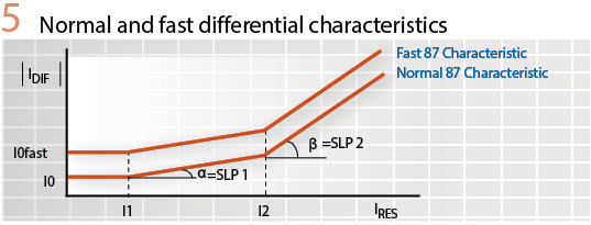
Use of shorter filter window times: Fast tripping times in EHV lines require the use of filter window times lower than one cycle. If the instantaneous differential and restraint currents are obtained, filter window times of one cycle and lower may be used at the same time. The use of both filters is normally required because fast filters, based on window times lower than one cycle, have higher transient overreach and they require a modified percentage differential characteristic (with a higher pick-up value, I0 as in Figure 5). If just the phasors at the fundamental frequency, calculated with a filter window time of 1 cycle, are interchanged between both line differential IEDs, the possibility of faster filters is removed.
Implementation of a line differential relay based on Sampled Values: Sampled Values (SVs) are multicast ethernet messages containing instantaneous values of voltage or current waveforms, not phasors. The new line differential relay is working at a communication speed of 2 Mbit / s (speed used with direct F.O. communication or with SDH at 2 Mbit/s) operates with instantaneous values sampled at 4800 Hz, the sampling frequency specified in IEC 61869-9 for protection applications. This allows the differential unit to operate with SVs interchanged between two substations.
Visualization of the remote current waveforms in the oscillography: If instantaneous values are interchanged between the line differential relays, the waveforms of both local and remote currents can be seen in the oscillography. This makes fault analysis easier.
Sending of current instantaneous values: As nowadays most of the communication channels used for line differential protection have a speed of 2 Mbit/s, the working sampling frequency of the line differential unit is decided to be 4800 Hz. This is the sampling frequency of ZIV e-NET FLEX family IEDs, as they have been designed to work with SVs. For lower speeds, such as 768 kbit / s (12 x 64 kbit / s with C37.94 communication protocol) or 64 kbit / s (PDH or 1 x 64 kbit / s with C37.94 communication protocol), downsampling to 1600 Hz and 800 Hz, respectively, is done at the transmission end, after applying a digital antialiasing filter. Upsampling to 4800 Hz is then done at the reception end.
The communication frame includes several instantaneous values, in order to make better use of the channel bandwidth. Each group of samples includes the time instant of the first sample (value going from 0 to 4799).
Time alignment of current instantaneous values: Synchronizing the sampling instants at both local and remote IEDs is important in order to remove false differential currents. Line differential IEDs include other units, apart from the line differential ones, such as distance, overcurrent, etc. These units work with local currents and their sampling cannot be defined by the remote end sampling, as communication disconnections and connections will make this sampling change continuously, affecting the operation of the mentioned local units. Therefore, the IED samples at 4800 Hz, but the sampling is not synchronized with the remote end one. For speeds lower than 2 Mbit/s downsampling to 1600 Hz / 800 Hz is done. New samples at 4800 Hz, time-aligned with the remote end, must be calculated at the local end. Polynomial interpolation is used for both upsampling (change from 1600 Hz / 800 Hz to 4800 Hz, when needed) and resampling (time-alignment of local and remote samples).
Resampling is based on the sampling instant of each sample (0 to 4799 instants), referred to the remote clock, and on the time-delay between the local and remote clocks.
After the samples at 4800 Hz, time-aligned, are obtained, a second resampling is done for frequency tracking, obtaining local and remote samples at 80 samples / cycle.
The polynomial interpolation is also used to estimate lost samples, in case communication frames are discarded because of channel errors.
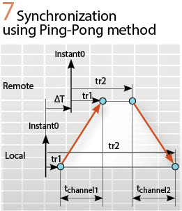
Calculation of the phase-shift between local and remote clocks: The delay between the time instants taken at both local and remote IEDs is calculated by means of the well-known “ping-pong” method (see Figure 7), interchanging messages and annotating time-tags.
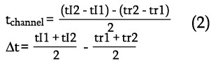
Assuming tchannel1=tchannel2=tchannel,
∆T and tchannel can be calculated as:
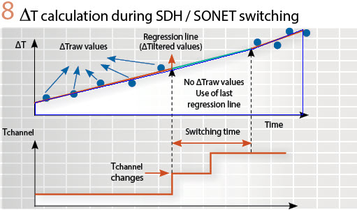
Once several ∆Traw values are obtained, a regression line based on least squares is used to calculate ∆Tfiltered values. This removes the influence of the channel jitter.
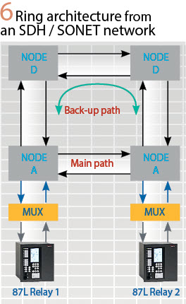
Errors coming from the synchronization method: Equations (2) were obtained assuming tchannel1 (going time) was equal to tchannel2 (return time), but SDH / SONET switching makes both times different. SDH / SONET networks normally work with ring architectures, as the one shown in Figure 6. Line differential relays 1 and 2 will usually communicate with each other (by means of SDH nodes A and B) through the shortest path (main path). When there is a failure in the main path (A-B / B-A) a switching to the back-up path (A-D-C-B / B-C-D-A) is done. The back-up path normally has a longer propagation time. Two types of switching can be applied: bidirectional, in which both paths, the going and return ones, are switched, creating transient asymmetries, as the switching of both paths does not occur exactly at the same time; unidireccional, in which only the faulted path is switched, generating permanent asymmetries.
Bidirectional switching: When a switching takes place, there is a change in the channel time. This change is detected comparing the channel time variation with the maximum expected jitter. Once the switching is detected, the clocks synchronization stops using new Traw values, as these values are not reliable due to the asymmetry. During the switching time, Tfiltered values based on the last regression line are used. This is shown in Figure 8.
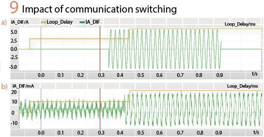
Figure 9.a shows a simulated bidirectional switching, the channel time increases 4 ms (first switch: going path) and, after 450 ms, it increases another 4 ms (second switch: return path). The switching time set in the relay is 200 ms, however the channel asymmetry lasts for 450 ms. 200 ms after the first channel switch the relay starts calculating new ∆Traw values and obtaining, after a number of values, a new regression line. This generates erroneous ∆Tfiltered values, which creates a false differential current. When the channel asymmetry is removed (450 ms after the first switch) and the regression line is updated, the differential current goes back to zero. The alignment errors create a phase-shift in the remote current.
The simulated bidirectional switching shown in Figure 9.a is repeated with an increased switching time setting, changed from 200 ms to 1 s. In this case, no new calculations of ∆Traw are performed during the channel asymmetry. This way, the alignment process is correctly done, as can be seen in figure 9.b. In this scenario the differential current is lower than 20 mA (the phase currents were equal to 10 A).
Unidirectional switching: The following methods can be applied to cope with unidirectional switching:
- External synchronization: both IRIG-B and PTP synchronization methods are included
- Directional comparison: if the angle between the local and remote currents is above a certain threshold the directional comparison will block the differential unit trip
- Robustness of the communication protocol and operation: The communication protocol of the line differential protection described in this paper is based on the well-known HDLC protocol. The new line differential relay includes many features that makes this communication protocol be robust to communication errors:
- Relay address to avoid accepting communication frames of other line differential relays
- Frame length checking to detect communication errors that modify the length of the frame such as erroneous bit stuffing, bit slips caused by clock drift, etc
- CRC of 16 bits which can detect theoretically more than 99.98% of the communication errors
- Redundant sequences which consist of inserting fixed patterns in the data frame. This sequence is checked at the receiver to detect bit changes and bit slips not detected in the previous checks
If SVs are used, the protection mechanism of the SV message is used.
Additionally, other security measures include the filtering on the activation of specific data, such as direct transfer trips and digital signals, that can be used for teleprotection. This filtering is implemented by making the digital signals to be received with the same status for a settable number of frames during a predefined window before accepting them. This way a compromise between security and dependability is obtained.
The interpolation mentioned above is also used to estimate lost samples. This can help if frames free of errors are received just after a few erroneous ones.
Another security measure is applied by supervising any differential unit trip by a fault detector, based on local measurements. This makes it invulnerable to communication errors. Both levels and variations in the local sequence currents are used to activate the fault detector. For weak infeed conditions, the voltages are checked.
Furthermore, the relay monitors the communication quality of each communication port by measuring the bit error rate (BER). Some statistics such Errored Seconds Ratio (ESR), Severely Errored Seconds Ratio (SESR) and Availability Ratio (ATR) are also provided.
Pure-Fault Differential Unit
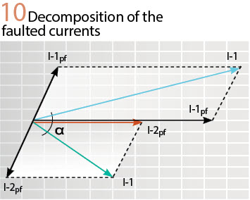
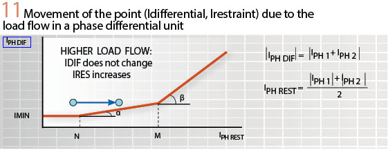
Because of the superposition principle, the faulted currents can be decomposed in prefault and pure fault currents (see Figure 10). The differential current is not affected by the load current, as the differential current tends to be zero during load conditions. However, the restraint current increases with the load current, as the load current increases the prefault restraint current.
The effect of the load for an internal fault is the movement of the point (Idifferential, Irestraint) to the right, therefore approaching the differential characteristic and reducing the dependability, as shown in Figure 11.
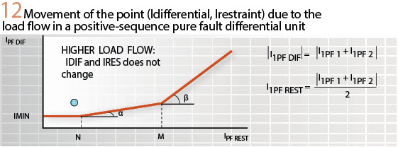
In the line differential relay described in this paper, a pure fault positive-sequence differential unit was added. This unit is unaffected by the load flow (see Figure 12, pf means “pure fault”), providing better sensibility.
The unit operates for any type of fault. On the other hand, as the pure fault restraint current is zero during prefault, the point (Idifferential, Irestraint) enters the operation area faster than in a phase differential unit.
The pure fault differential unit is blocked by the same external fault detector (based on the idif/ires ratio and on directional comparison units) that blocks the phase differential unit, therefore it provides the same security. It can also trip single-pole thanks to a phase selector.
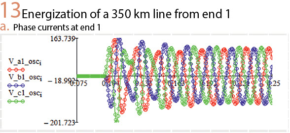
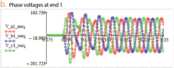
Capacitive Current Compensation
The line capacitance generates a differential current that can be compensated if the phase voltages are measured and the positive and zero-sequence line capacitances are known. As the line differential relay described in this article calculates the differential current based on instantaneous values, the capacitive current is also calculated with instantaneous values.
This calculation provides better accuracy during transient conditions, including frequency components different from the fundamental one, than the calculation based on phasors. The capacitive current is calculated with the following formula:
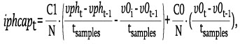
Where:
- vph: is the instantaneous phase voltage
- v0: is the instantaneous zero-sequence voltage
- tsamples: is the time between samples
- C1: is the positive-sequence line capacitance
- C0: is the zero-sequence line capacitance
- N: is the number of ends capable of doing capacitive current compensation
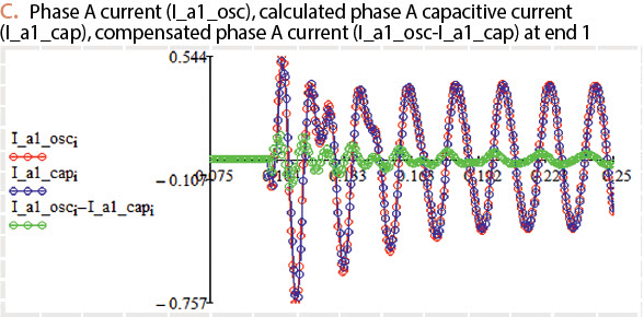
A compensated phase current is calculated as:
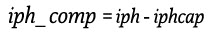
Each IED sends the compensated phase current to the remote end.
Figure 13 (a/b/c) shows the phase currents and voltages during the energization of a 350 km 220 kV line, simulated with an RTDS. Figure 13 shows the phase A current, the calculated phase A capacitive current and the compensated phase A current. As it can be checked the compensated current is practically zero. It is not exactly zero because the capacitive current is calculated with a PI circuit, while the line is modelized with a distributed parameter circuit. Nevertheless, the difference in the compensated current generated by both models is very low.
Biographies
Roberto Cimadevilla graduated in Electrical Engineering from the Higher School of Engineering of Gijón, Spain in 2001. He did his final year project at the University of Dundee, Scotland, and obtained a master´s degree in “Analysis, simulation and management of electrical power systems” at the University of País Vasco, Spain. He started his professional career in the protection maintenance area of Red Eléctrica de España (Spanish TSO). Roberto joined ZIV in 2003, where he actively participated in the development of several protection and control devices, including distance, transformer differential, line differential and feeder relays. Roberto has held several positions of technical and management responsibility inside ZIV. He is currently the Manager of the Application Engineering Department of the T&D Product Line. Roberto has written more than 25 papers, he is an IEEE member and has participated in several CIGRE working groups.
Javier Garcia-Villalobos received the Automatic and Industrial Electronics Engineering degree and the Integration of Renewable Energies in the Electrical System master’s degree from the University of the Basque Country, Spain, in 2010 and 2011, respectively. He obtained the PhD degree from the University of the Basque Country in 2016. Javier joined ZIV in 2017 as Application Engineer and Project Manager. He has published several journal papers and book chapters. Also, he has presented/participated in more than 20 conference papers. Currently, his research interests are related to the electrical power system monitoring, analysis and protection.